Overview
In computer graphics and game development, matrix transformations are an esential topic in order to manipulate the movement of the objects in the 3D world. Since these objects are composed by vertices, we just need to modify their values to reproduce different kind of movements like moving the object at an arbitrary point, rotating it around itself or scaling it up bigger or viceversa.
So all this means, in technical terms, that we need to perform a set of 3D transformations on the objects by using matrices as is the optimal way to work to apply these transformations to each one of the vertices that compose every object of the 3D World.
Each matrix is responsible for a single transformation in the process and will be applied to each vertex of the object in order to perform the respective transformation.
This means that we have three matrices: translation, rotation and scaling transformation, and we want to apply them one by one on the position vector.
Matrix Fundamentals
Combination of matrices
Besides, matrices can be multiplied together in order to combine all the transformations into a single matrix. Notice that we have to construct the matrices in a way that they must be multiplied on the left-hand side of the vector.
This may look something like this:
Parentheses order doesn't matter
Based on the associativity of matrix multiplication law, in linear algebra the placement of parentheses in a secuence of matrix multiplications doesn’t change the final result.
This is important in terms of a performance point of view since we don't need to provide multiple matrices to the GPU and apply them one by one on each vertex. We can multiply them once in the software and simply provide the result of the multiplication to the GPU to perform a single matrix-vector multiplication.
Multiplication order matters
Based on the non-commutativity of matrix multiplication law, in linear algebra if we change the order which we multiply the matrices, we may get a different result.
So the order is critical in terms of what we are trying to achieve. Translation * Rotation is not the same as Rotation * Translation. The first one will spin the object around itself placed in an arbitrary point and the second one will spin the object around an arbitrary point.
Same behaviour happens wiht these matrix-vector multiplications where the matrix is on the left-hand side because in matrix-vector or matrix-matrix multiplication, we do a dot product between a row on the left and a column on the right.
We could have placed the vector on the left, but this would have required us to put the translation vector on the bottom row of the matrix rather than on the rightmost column.
Matrix Class
Matrix layout
When developing the matrix class as a storage of 16 floating point values representing the 4x4 matrix, its important to notice how we are organizing these values in terms of memory storage as graphics APIs have 2 manners to read and interpret the matrices composition when we send them to the GPU.
-
Row-major Order: In row-major order means we are supplying its values first along its rows, and when the row is complete, we move to the next one. -
Column-major Order: In column-major order, we go first down along the column and then continue to the right to the next column.
In both cases, we start with the top left-hand corner.
In the following matrix class, we choose to storage the 16 data values as a 1D-array and treating them using the column-major order. The class is a partial specification of the template class Matrix where we can configure the underlying data type of the matrix. As you will se later, we will handle it with floating point values.
    template< std::uint8_t, std::uint8_t, typename T >
    class Matrix;

    template < typename T >
    class Matrix<4,4,T>
    {
    public:

        // 16 type value storage
        T m_Mat[16] {};
        std::uint8_t m_Rows {4};
        std::uint8_t m_Cols {4};

        // column-major order matrix layout
        constexpr explicit Matrix() noexcept
        {
            for (int i {0}; i < m_Rows; ++i)
            {
                for (int j {0}; j < m_Cols; ++j)
                {
                    m_Mat[i * m_Rows + j] = 0;
                }
            }
        }
    };
We can add helper constructors and methods to initialize the 1D array with a default state. For example, to build the identity matrix.
    constexpr explicit Matrix(const float value) noexcept
    {
        for (int i {0}; i < m_Rows; ++i)
        {
            for (int j {0}; j < m_Cols; ++j)
            {
                m_Mat[i * m_Rows + j] = (i == j) ? value : 0;
            }
        }
    }

    constexpr void Identity() noexcept
    {
        for (int i {0}; i < m_Rows; ++i)
        {
            for (int j {0}; j < m_Cols; ++j)
            {
                m_Mat[i * m_Rows + j] = (i == j);
            }
        }
    }
In order to make the code easier to read and mantain, we can define an alias for the total specialization of the matrix template class using floating points as the underlying data type.
using Matrix4 = Matrix<4, 4, float>;
Matrix Multiplication
Probably the most important matrix operation that we have to build is the multiplication one as matrix multiplication is totally esential in order to apply transformations in computer graphics.
The following code is one of many approaches to archieve a matrix-matrix multiplication, which doesn't mean to be the best one, just the one I crafted.
    Matrix operator*(const Matrix& other) const
    {
        Matrix result {};

        // row left & result matrix
        for (int k = 0; k < m_Rows; ++k)
        {
            // col right matrix
            for (int i = 0; i < m_Cols; ++i)
            {
                auto& resultElement = result.m_Mat[(i * m_Cols) + k];
                // row right matrix
                for (int j = 0; j < m_Rows; ++j)
                {
                    auto& e1 = m_Mat[(j * m_Cols) + k];
                    auto& e2 = other.m_Mat[j + (i * m_Cols)];

                    resultElement += e1 * e2;
                }
            }
        }

        return result;
    }
With this introduction and basic matrix class implementation, we can jump into the matrix transformations and how to implement them in the matrix class!
Translation Transformation
The first transformation that we will talk about is translation, which means the placement of an object to an arbitrary point in the 3D world. In order to move the entire model around completely, we have to apply the same translation to the position of the all model vertices.
At first glance, it seems quite straightforward.
We can specify the translation along the X, Y, and Z axes in a 3D vector called translation vector and perform a component-wise addition
of the position vector and that translation vector.
Translation Matrix
As we said before, we usually work with matrices in order to apply these transformations. So, we need to represent this component-wise addition in a matrix format.
In order to transform a position vector by a matrix using the dot product as the core operation in a matrix vector multiplication,
we need to add a 4th row in position vector with the value of 1 called W
and using a 4x4 matrix where we place the translation vector in the 4th column.
If the other columns are represented like an identity matrix, through the dot product multiplication we can preserve both position components and translation components to finally apply the component-wise addition.
Graphics APIs like OpenGL were designed taking into account this kind of calculations and
that's the reason why graphics system variables are constructed as 4D vectors called as
homogeneous coordinates.
Code
The following code is an implementation of a translation transformation where we define a new matrix method called Translate() that recieves a 3D vector as a parameter.
This parameter means the translation vector, which is applied in the local generated matrix to represent the translation matrix.
Once we have the translation matrix, we just need to perform the matrix-matrix multiplication with the new overwritted multiplication operator.
    void Matrix::Translate(const Vector3& aTranslation)
    {
        // Creates an arbitrary matrix
        Matrix4 TransMat {};

        // Set up as an identity matrix
        TransMat.Indentiy();

        // Set the translation vector into the matrix
        TransMat.SetTranslation(aTranslation.x, aTranslation.y, aTranslation.z)

        // Apply the translation by matrix multiplication
        auto& MatRef = *this;
        MatRef = TransMat * MatRef;
    }
SetTranslation() is a private method that sets the translation values into the 4th column:
    void Matrix::SetTranslation(float aX, float aY, float aZ)
    {
        m_Mat[12] = aX;
        m_Mat[13] = aY;
        m_Mat[14] = aZ;
    }
In the Scene, we just need to use the Translate() method in order to move an object to a location.
In the example, we use a delta floating factor that goes through X axis domain.
    void Scene::OnUpdate()
    {
        // Incrementing delta value through X axis...

        // (1) Setting up WizardMat with translation transform
        Matrix4 WizardMat {};
        WizardMat.Identity();
        WizardMat.Translate(Vector3{delta, 0.f, 0.f});

        // (1) Send WizardMat to the GPU...
    }
If we run the sample code in our scene, we get something like this:
Rotation Transformation
Let's talk now about rotation transformations, which means that the object rotates or spins. It can be around itself or it can be in a combination with translations, so first you can move it and then it rotates around some external point.
Angle-Axis rotation
The basic rotation is around one of the three cardinal axes of the coordinate system: around
X,
Y, or
Z.
Therefore, we can apply them one by one on the model so that eventually it will rotate around all the axes as we are chaining them.
This means that when we are rotating around the X axis, we are actually moving on the plane that is created by the other two axes, the Y and the Z. Our location on the X axis remains constant and our location on the Y and Z changes.
Notice that the core rotation seems equivalent across the three axes as we are applying similar behaviour.
This means that we can develop the equation on one case in Z axis and apply it with minor changes on the other cases with X and Y axis.
Coordinate Rotations
In this article we will calculate the transformed coordinates around an arbitrary axis using the trigonometry functions and identities without taking into account the polar coordinate's approach. The approach we will use can be based on rate of movement in rotations.
Each frame is a step where we are applying an angle value as a delta step in order to calculate the transformed coordinates of the point along the circle.
let's say that our starting position is located at x1 y1, which is at angle alpha from the X axis, and we want to move from this location counterclockwise by the angle of beta. So we want to calculate x2 and y2.

Notice that in computer graphics, the standard convention is that counterclockwise movement is positive in terms of the angle and clockwise movement is negative.
Taking into account that in mathematics we have to start from one axis point in order to rotate, the trigonometry equations will be something like that:
Following the analogy, we can get the transformed x1 and y1 with the sum of angles:
To apply the sum of angles, we need to use to following handy trigonometric identity that we can use to calculate sine and cosine of sums of angles:
With the previous trigonometry functions, we can get the following formula where we have as inputs the starting position at (x1,x2) and the angle of rotation beta and outputs the transformed position at (x2,y2):
Rotation Matrix
If we take the transformed X and Y from these equations, Z remains in whatever value it had originally, and W is always 1, we can write this down as a vector:
With the vector format, we can actually represent it as a multiplication of a matrix by a vector as you can see below.
We moved everything which is related to the angle of beta into a matrix and in the vector we just have the original position X, Y and Z. Thus, this is the rotation matrix around the Z axis.
Since the rotations around all three axes are virtually equivalent, it is very easy to construct the rotations around X and Y in a similar fashion.
Code
The following code is an implementation of a rotation transformation around Z axis where we define a new matrix method called RotateZ()
that recieves a floating point value as a parameter.
This parameter represents the angle of beta, which is applied in the local generated matrix to represent the rotation matrix.
Once we have the rotation matrix, we just need to perform the matrix-matrix multiplication using the new overwritted multiplication operator.
    void Matrix::RotateZ(const float aAngle)
    {
        // Creates an arbitrary matrix
        Matrix4 ZRotMat {};

        // Set up as an identity matrix
        ZRotMat.Indentiy();

        // Set the rotation angle into the matrix
        ZRotMat.SetRotationZ(aAngle);

        // Apply the rotation by matrix multiplication
        auto& MatRef = *this;
        MatRef = ZRotMat * MatRef;
    }
SetRotationZ is a private method that performs the trigonometry functions using the input angle and sets the result into the rotation matrix.
As you could see, we have to work in radians because we are going to plug it into the sine and cosine functions of the C standard library which expects the angle to be in radians rather than degrees.
Remember that a single radian is about 57.3 degrees!
    void Matrix::SetRotationZ(float aAngle)
    {
        const auto radAngle {static_cast(aAngle * PI / 180.f)};

        m_Mat[0] =  cosf(radAngle);
        m_Mat[1] =  sinf(radAngle);
        m_Mat[4] = -sinf(radAngle);
        m_Mat[5] =  cosf(radAngle);
    }
In the Scene, we just need to use the RotateZ method in order to rotate an object around the Z axis.
In the example, we use a delta angle value to rotate both clockwise and counterclockwise directions.
Remember that in the rasterizer the X axis is horizontal, the Y is vertical and the Z simply goes into and out of the screen so we expect the object to rotate around it.
    void Scene::OnUpdate()
    {
        // Incrementing and Decreasing delta angle value...

        // (1) Setting up WizardMat with rotation transformation
        Matrix4 WizardMat {};
        WizardMat.Identity();
        WizardMat.RotateZ(delta);

        // (1) Send WizardMat to the GPU...
    }
If we run the sample code in our scene, we get something like this:
Scaling Transformation
Finally, we have the scaling transformation to scale up the model and make it bigger or the other way around, scale it down and make it smaller. Scaling transformation multiplies one or more components of the position coordinates by an arbitrary factor.
-
Non-uniform scaling: When scaling transformation only modify one dimension or when the scaling factor is different for each dimension, we call this “non-uniform scaling" and original proportions of the object are lost. -
Uniform scaling: When scaling transformation modifies all dimensions with same scaling factor, we call this "uniform scaling" and it preserves the proportions of the object.
If the scaling factor is greater than one, the object becomes larger. If it is less than one but greater than zero, the object becomes smaller.
Notice that if the scaling factor is negative, the object flips.
Scale Matrix
To represent the vector position scaling by a matrix-vector multiplication, all we have to do is replace the value of one with the desired scaling factor for this position in a identity matrix.
Performing a scaling transformation is pretty straightforward since the dot product of each row by the corresponding components of position vector accomplishes the requirement of component-wise multiplication by the scaling factor to scale up/down the position coordinates.
As we said before, if the three scaling factors are identical, this is a uniform scaling matrix. If they are not identical, then this is a non-uniform scaling matrix.
Code
The following code is an implementation of a scaling transformation where we define a new matrix method called Scale()
that recieves a 3D vector as a parameter.
This parameter represents the scaling factors for each component of the position vector, which are applied in the local generated matrix to represent the scaling matrix.
Once we have the scaling matrix, we just need to perform the matrix-matrix multiplication using the new overwritted multiplication operator.
    void Matrix::Scale(const Vector3& aScale)
    {
        // Creates an arbitrary matrix
        Matrix4 ScaleMat {};

        // Set up as an identity matrix
        ScaleMat.Indentiy();

        // Set the scaling factors into the matrix
        ScaleMat.SetScale(aScale.x, aScale.y, aScale.z);

        // Apply the scaling by matrix multiplication
        auto& MatRef = *this;
        MatRef = ScaleMat * MatRef;
    }
SetScale() is a private method to set the scale factor values into the diagonal matrix slots.
    void Matrix::SetScale(float aScaleFactorX, float aScaleFactorY, float aScaleFactorZ)
    {
        m_Mat[0] =  aScaleFactorX;
        m_Mat[5] =  aScaleFactorY;
        m_Mat[10]=  aScaleFactorZ;
    }
In the Scene, we just need to use the Scale() method in order to scale up/down an object.
    void Scene::OnUpdate()
    {
        // Incrementing and Decreasing scaling factor values...

        // (1) Setting up WizardMat with scale transformation
        Matrix4 WizardMat {};
        WizardMat.Identity();
        WizardMat.Scale(Vector3{delta, delta, 0.f});

        // (1) Send WizardMat to the GPU...
    }
If we run the sample code in our scene, we get something like this:
Projection Transformation
Now it's time to introduce us into the world of 3D as our physical world is obviously 3D and objects have a depth.
In real world, we percieve sense of distance to objects really well as objects further away from us appear to be smaller and vice versa, so we espect 3D games to be the same way. The problem is that when we change the depth of the objects (Z axis), they appear to look the same as they are same size on the screen.
Computer graphics doesn't do this job automaticaly, so it's our job to change their size based on distance.
We will se why it's important the role of 4th component W in the vertex position since it is used for 3D and perspective projection.
Rasterizer Issue
A vertex to be rendered on screen needs its X and Y components to be within the [-1,-1] to [1, 1] range, otherwise the rasterizer will simply clip it away. We can manipulate the values in GPU with a few transformations (translation, rotation and scaling) but when the vertex has reached the rasterizer, its over.
We can not change the X and Y values and the rasterizer will simple render the triangle based on the X and Y of the three vertices.
So, in order to archieve the illusion of 3D we have to tweak the X and Y values so that the triangle will appear to be bigger or smaller based on its distance from the camera.
This transformation is called perspective projection.
Frustum View
It all begins with the concept of frustrum view. Frustrum view is a simplified concept of the human eye model and it represents the visible part of the 3D world.
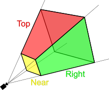
It's not recommended to match the human eye too precisely because it will simply make our calculations much more complex and the benefit will probably be not that great. After all, we are rendering into a rectangular window and our vision is clearly not rectangular.
Everything inside the frustum will be rendered in our window and everything else will be partially or completely clipped away. The frustum itself has four sides that represent the extent of the viewable volume of space in terms of the horizontal and vertical width.
These sides are represented as clip planes because everything that cuts through them is clipped.
- Top & bottom clip planes
- Left & Right clip planes
Near and Far clip planes
In addition to that, we have a couple of more clip planes that need an more in-depth introduction:
- Near clip plane
- Far clip plane
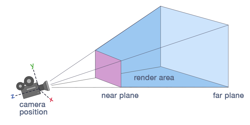
These additional planes appear as the imposibility to approach our human eye model since we are not limited in terms of the distance to the light origin. We can see stars that are light years away if their light is bright enough.
In 3D computer graphics, we want to reduce the amount of compute required to render the scene and by clipping away objects that are far away
from the user, we help reduce the load on the system.
In addition we dont want to deal with large numbers because of numerical issues that such numbers introduce as we capture the Z value
in a buffer called Depth Buffer for depth testing.
In the view frustum, we use the far clip plane in order to limit the maximum distance to the triangles that can be rendered.
This will affect the way the user will perceive the environment in terms of the distance to the horizon as well as the precision of the depth
buffer which can get you into a critical problem called Z fighting.
Near clip is pretty important too since it is set to go from -1 by -1 at the bottom left, to 1 by 1 at the top right in order to match with the rasterizer size and map each 3D point from the virtual 3D world to actual pixels into the plane. As the clip plane matches with the rasterizer in terms of proportional size, the projected point in the near clip is exactly the coordinate that we need to specify to the rasterizer in order to render the original 3D point.
Frustum view usage:
- Clipping out stuff outside of the scene.
- Limit maximum distance to avoid precision issues.
- Project 3D points into pixels taking into account rasterizer normalized squared size.
3D Illusion method
Firstly, let's assume for simplicity, that the camera is located at the origin of the coordinate space and it is looking straight down along the positive Z axis.
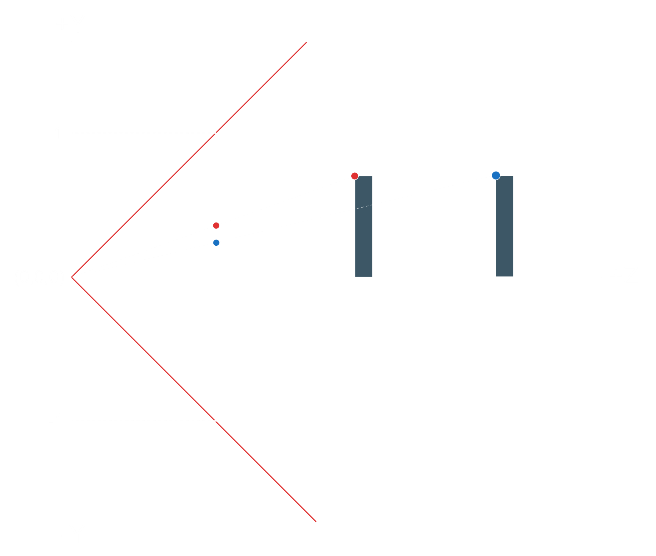
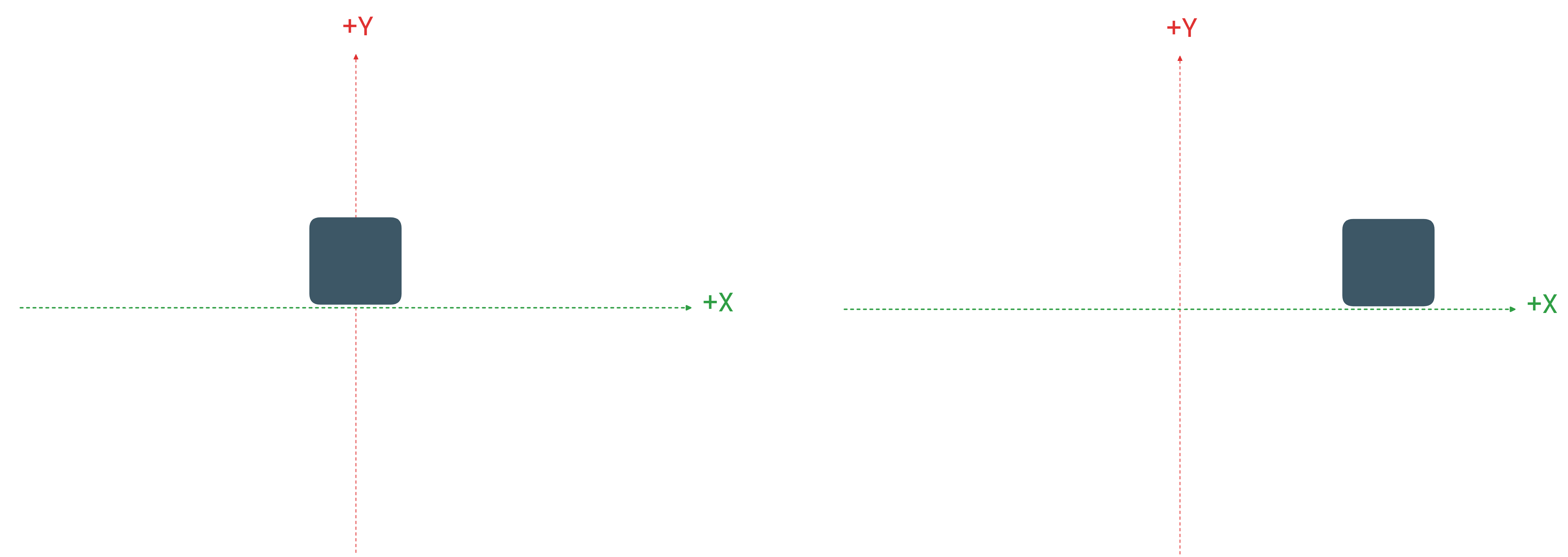
In order to accomplish the illusion of 3D, we can see that if we put two boxes with different distances from the camera and project a vertex of both boxes to the origin, even though the boxes are identical, the intersection points are different.
Using this method to render all the triangles of the two boxes, we will see that the closer box appears to be larger than the one which is more distant.
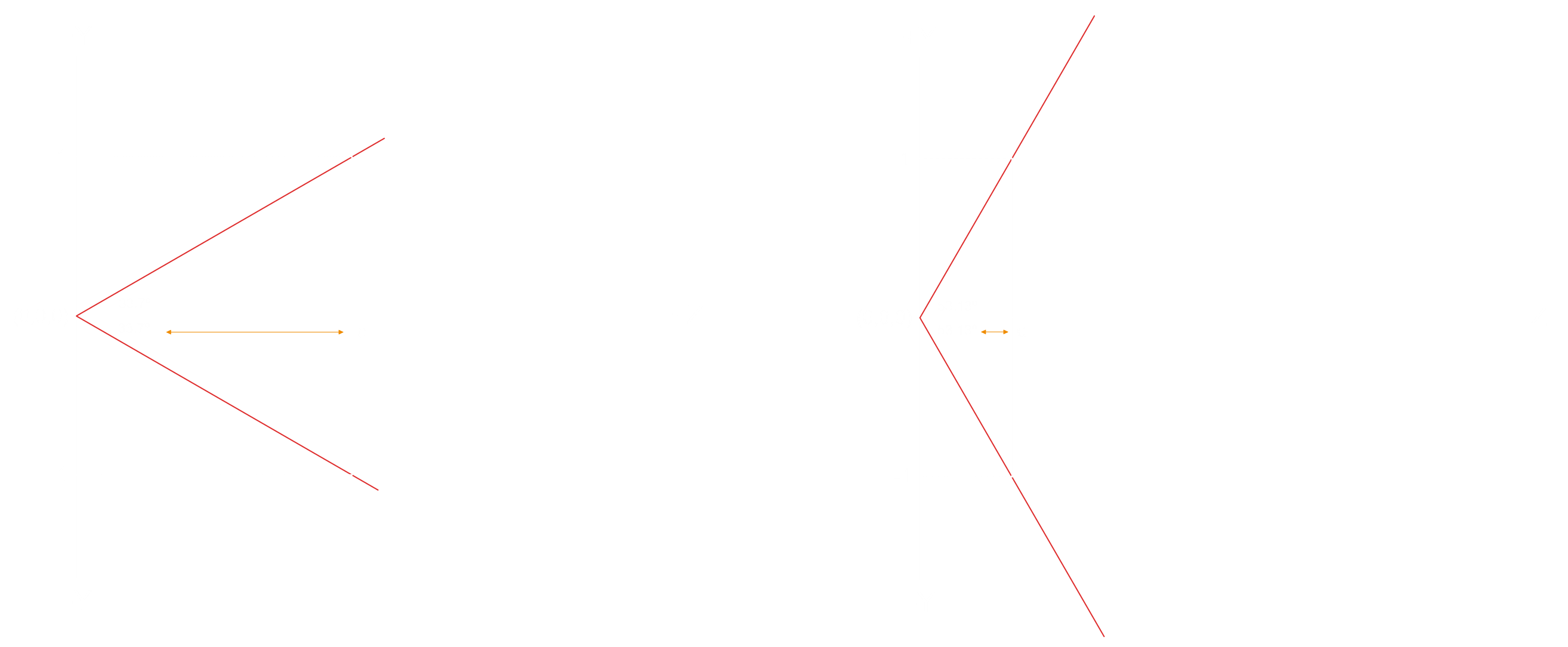
FOV
As we put the camera at origin (0,0,0), the near clip plane can be placed at any distance from it.
This distance is based on an angle between top and bottom planes of the frustrum and its called the vertical field of view.
Decreasing the value of this angle, we can move the near clip plane away from the origin which would decrease the viewable vertical range
so the objects will appear to be larger in the screen (zooming in).
Increasing the value of the angle, we would move near clip plane closer to the origin which will gain viewable vertical range and objects
will appear to be smaller (zoom out).
Same behaviour with the horizontal field of view as the ratio between them should match the ratio between the window height and width. Otherwise, the image will appear to be stretched one way or the other.
Projection Coordinate System
3D Point Projection
Now that we know that we need to map any 3D coordinate to some point on the near clip plane which matches the rasterizer range in the X and Y axes, that is from -1 to 1, it's time to calculate the location of the projected 3D point on the near clip plane!
We want the user to control the field of view so in general let's call this angle alpha.
We can actually divide alpha into two halves, above and below the Z axis.
Since the field of view is configurable, the distance to the near clip plane is denoted as 'd'.
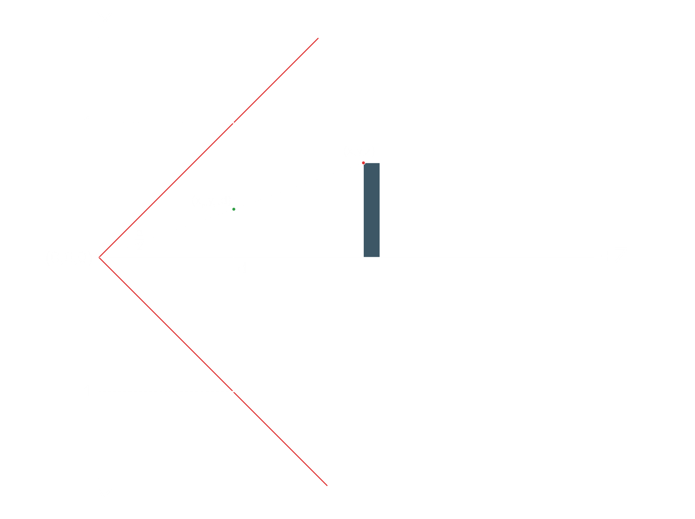
We can calculate d using the tangent trigonometry function:
Given the red point which has a 3D position (X,Y,Z), we want to find the location of the green point which is the projection on the near clip plane. The Z value of the green point is obviously d, same as the near clip plane.
We will do a similar trick from the top and calculate the Xp in the exact same way.
Right now we are focusing on Yp.
Similar Triangles Ratio
If we pay attention to the previous image graph, we can observe that there are two diffent triangles formed by the projection of the 3D point. Each of them with different distances in the Z axis but same angle. The fact that they are similar provides us with the equation of similar triangles ratio:

Using this equation, we can get the Yp:
So we have found the projected Y coordinate and finding the Xp coordinate is exactly the same.
This time we are looking from the top down at XZ plane.
The vertical field of view angle is again alpha because we are using a square near clip plane to match the rasterizer range of coordinates.
(We'll take care of the aspect ratio later).
As you can observe, we used the same equation to calculate the distance to the near clip plane d.
The equation that calculates Xp is also the same as the one for the Y so we just need to replace X with Y all over the place.
Finally, we get the projected Xp and Yp equations:
Aspect Ratio
Right now, we have a square window. If you try to use a rectangular window, which is wider than tall, then you will see that the image becomes stretched. So we need to provide some solution there.
The rasterizer was designed as fixed-function hardware that has less room for configurability so we have to cook a solution in software
as the GPU use a square rasterizer that goes from -1 to 1 on both X and Y.
This rasterizer kind of sits in the middle of the whole transformation procedure because when we reach the rasterizer square coordinates
after all the trasnformations, we have to apply something called a viewport transformation
in order to convert the clip space coordinates to window coordinates that match the window that the user created.
To take into account the forthcoming transformation to viewport space coordinates, we simply need to divide the projected X value by the aspect ratio. This is straightforward to understand:
For instance, if we have an aspect ratio of 2 (2000p width and 1000p height), it means that we have twice as many horizontal pixels as vertical ones, causing objects to stretch horizontally. To counteract this, we divide the projected X value by 2 to compensate the horizontal stretch.
On the other hand, with an aspect ratio of 0.5 (1000p width and 2000p height), objects would vertically stretch to fill more vertical pixels. As we divide the projected X value by the 0.5 aspect ratio, we're effectively doubling X, thus compensating for the vertical stretch by horizontally stretching the objects.
With this approach, after the viewport transformation, we will get the right results since in reality, we are remapping the viewport space points into the rasterizer space points as we are condensing all points along the X axis.
Example of aspect ratio equation with an HD Window size:
Z Transformation
Let's talk about the Z value. We're going from 3D coordinates down to 2D coordinates on the screen, so why do we even care about the Z value?
When we perform a projection of a 3D coordinate to 2D coordinate on the screen, we can have potentially an infinite number of pixels with different Z values that are projected into that 2D coordinate pixel and we want to make sure that we render the one the one which is the closest to the camera. This problem appears when there are overlapping objects.
Depth Test Algorithm
The solution used in the graphics APIs is using the depth test algorithm and store the Z value of each pixel in what is called a
depth buffer.
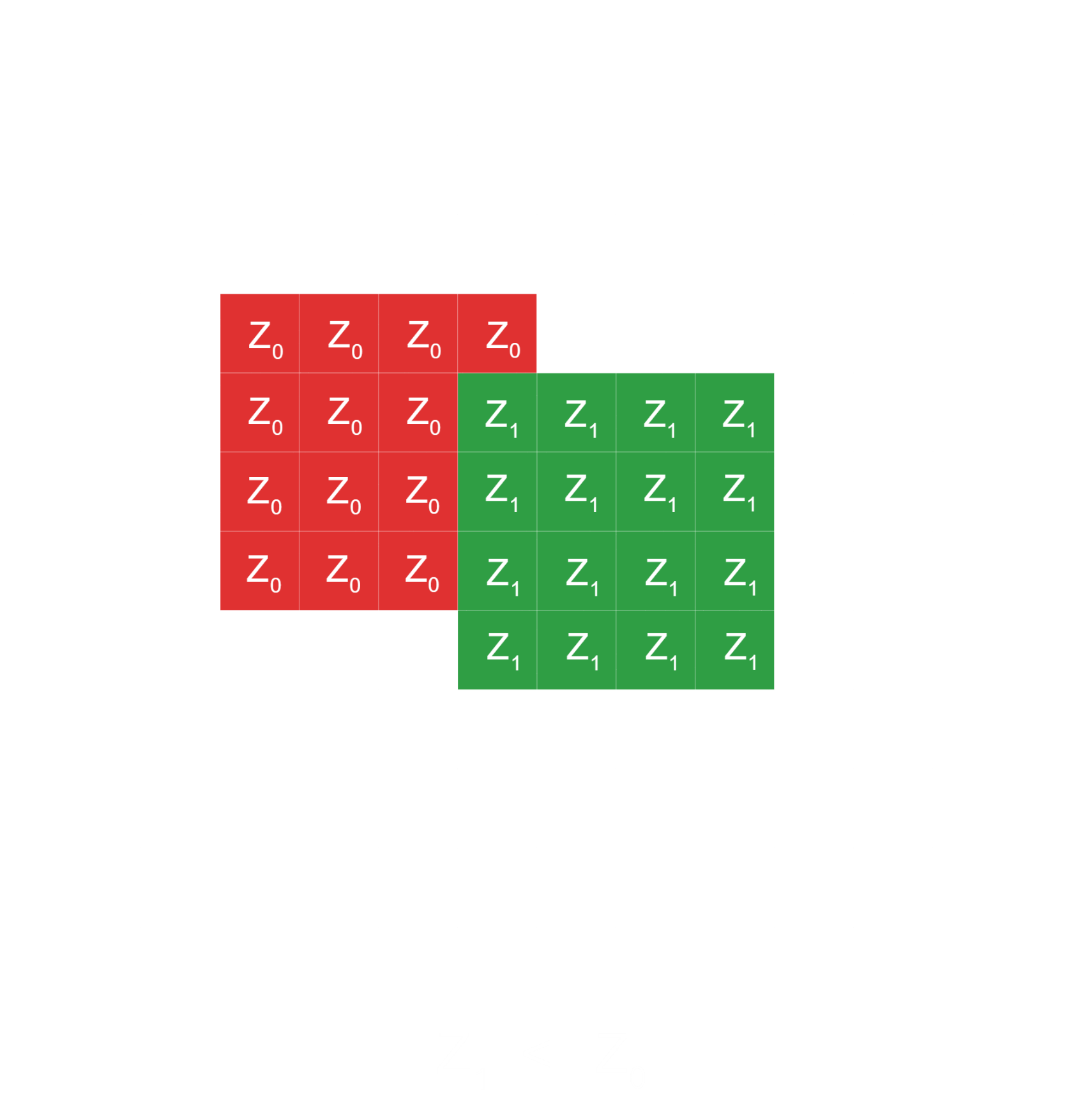
The resolution of the depth buffer is identical to the color buffer, so for every pixel cell in the color buffer, there is a corresponding cell in the depth buffer. The depth buffer is initialized with the largest Z value in all cells, and on every incoming pixel, we perform a depth test. We compare the incoming pixel's Z value with the one in the depth buffer.
If the incoming Z value is smaller than the one in the buffer, we render the color of the incoming pixel, and we overwrite the value in
the depth buffer with the incoming pixel's Z value.
If it is the other way around, the pixel is more distant, then we simply discard it and we don't do anything.
The system actually supports multiple comparing conditions, such as less than, less than or equal, etc.
Depth Test Precision Issue
In computer graphics, the results given by this approach are not that great at all as we encounter a problem during the depth test algorithm. The problem is the way the values of a floating point number are distributed across the 32 bits that we have in order to store it.
Since floating point numbers have 32 bits, the number of permutations that can fit in 32 bits are from zero to almost 4.3 billion, or 2 to the power of 32 minus one and that's exactly the number of permutations that we have to represent in floating points values from negative infinity to positive infinity.
This is very limited in terms of the precision that can be achieved. So, back in 1985, the designers of the IEEE 754 specification decided to distribute the floating point values in a way that most of them are within the -1 to 1 range, providing the greatest precision in that range.
As we go outside of this range, the precision starts dropping. In fact, half of the available bit permutations, about 2 billion, are used by the -1 to 1 range. And we have another 2 billion for everything else. This means that, in general, when dealing with floating points, you should strive to keep your core calculations within the normalized range and scale up for the final result.

As a result of this, graphics designers decided that the depth buffer will store Z values from -1 to 1, and everything outside that range
will be clipped. This means that, we will need to map our original Z values to -1 to 1.
Specifically, the near clip plane will be mapped to -1, and the far clip plane will be mapped to 1.
Precision Drop Issue
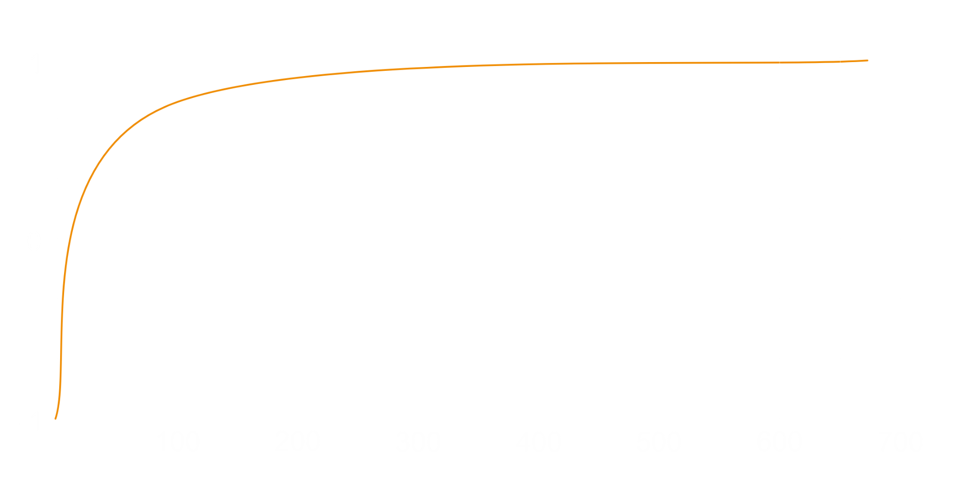
If we map a range between 1 and 100 using steps of one-tenth into normalized range [-1, 1] using the equations that will transform the Z values
into a normalized range that will be developed later, we can get a plot where we see a nonlinear mapping between the original Z range
and the transformed Z range due to the division by Z.
The best precision is achieved when the original Z is below 20, but as Z grows higher, the precision drops, and many values are mapped to very close values in the transformed Z range. So, the thing is that we should kept the Z range as tight as possible.
Z Transformation equations
Now we know that we need to normalize the Z values of each vertex in the scene to align them with the depth buffer storage format.
In order to transform them, we have to establish a relation of minimum and maximum Z values in the scene with the [-1, 1] range where the transformed NearZ has to be -1 and transformed FarZ has to be 1.
The third row is the responsible to modify the Z component of the position vector taking into account the dot product procedure, so we set the constants
[C, D, A, B] that we need to obtain.
As we have to do nothing for X and Y components, we can put zero in C and D.
So, the equation of Zp remaing as the following:
As we know that the rasterizer will perform later a Z division, we can apply it to the equation:
Now, we replace Z with the the minimum and maximum Z's of the scene in relation of the [-1, 1] normalized range. So the Zp output values have to be -1 for the NearZ value and 1 for FarZ value.
In the NearZ equation, we isolate A constant:
Once we have A isolated, we can replace the equation into the FarZ one and then we can obtain B constant as is the unique incognite there:
Using the common denominator and a bit of basic maths, we simplify the B equation a little bit.
A little shuffle to isolate B and we get the following B equation:
With B solved, it's so straightforward to solve A. We just need to replace the B equation into the last A isolation equation and use again the common denominator to obtain A.
Thus, we got the Z transformation equations:
Projection Matrix
Basic Perspective Projection Matrix
With the two equations that allow us to calculate the coordinates that the rasterizer needs to render, we could implement them directly in the GPU. 3D coordinate can be given to us as input attribute and the tangent of half fov angle can be calculated once outside the shader and provided as a uniform.
The problem is that this will be a waste of GPU cycles and we can simply create yet another matrix for this equations.
This matrix is called the projection matrix.
We don't want to add anymore transformations after the projection matrix since the projection matrix calculates the actual coordinates that the rasterizer needs to render on the screen.
When creating the matrix composed of the Z equations, we run into a problem. We still need to divide both X and Y by the Z value and there is simply nothing that we can put into the projection matrix that will divide by a component of the vector that is multiplied by this matrix.
Notice that the matrix has to be generated only once and used to transform multiple position vectors. So, this matrix has to be independent of vertex coordinates.
Perspective Division Stage
The 3D pipeline architects were fully aware of this problem and the idea that they came up with
was to add a fixed function stage in the rasterizer that will take gl_Position vector which is coming out of the vertex shader
and divide it by the W coordinate.
That's why we need a 4th component! (Z component could not be used because it would be transformed so the original value will be lost).
The trick then is to copy the original Z value into W and the rasterizer will divide by W which of course contains the Z value.
This stage is called perspective division and it cannot be turned off.
This is very simple to archieve using the following minimal change in the projection matrix:
That's not at all completed projection matrix as we still have to add the aspect ratio and Z transformation equations.
Projection Matrix - Aspect Ratio
Taking into account the aspect ratio equation:
We just need to add the aspect ratio equation into the projection matrix in the Xp component:
Projection Matrix - Z Normalization
Taking into account the Z transformation equations that we developed before:
If we replace the equations to the A and B constants that represents the part of the matrix that modifies the Z value of the vector, we can say that we finally get the projection matrix!
Code
The following code is an implementation of a perspective projection transformation where we define a new matrix method called Perspective()
that recieves a set of perspective inputs as parameters.
The FOV to calculate the projected Xp and Yp equations, the aspect ratio to take into account the viewport non-squared size and the far and near Z's to normalize the Z values into a normalized range for the depth buffer.
These input parameters are passed through the private method SetPerspectiveProjection() to build the projection matrix which has been created locally.
Once we have the perspective projection matrix, we just need to perform the matrix-matrix multiplication using the new overwritted multiplication operator.
    void Matrix::Perspective(float fov, float aspectRatio, float nearClip, float farClip)
    {
        // Creates an arbitrary matrix
        Matrix4 ProjectionMat {};

        // Set up as an identity matrix
        ProjectionMat.Indentiy();

        // Build the perspective projection matrix based on FOV, aspect ratio and Z ranges (near, far)
        ProjectionMat.SetPerspectiveProjection(fov, aspectRatio, nearClip, farClip);

        // Apply the perspective projection by matrix multiplication
        auto& MatRef = *this;
        MatRef = ProjectionMat * MatRef;
    }
SetPerspectiveProjection() is responsible of calculate the distance of the near plane based on FOV input value, treated in radiants, and put the Xp and Yp equations
into the matrix. Besides, adds a value of 1 to save the original value of Z in the W component of the vector and calculates the A and B equations to transform the Z value.
    void Matrix::SetPerspectiveProjection(float fov, float aspectRatio, float nearClip, float farClip)
    {
        // Calculate 'd' distance to near plane based on FOV
        float halfFOV       {aFOV / 2.f};
        const float radFOV  {static_cast((halfFOV * PI) / 180.f)};
        float tan           {tanf(radFOV)};
        float d             {1.f/tan};

        // Map X & Y values to transformed X,Y [-1,1]
        // We take into account different aspect ratio to match rasterizer aspect ratio of 1
        m_Mat[0] =  d / aAspectRatio;
        m_Mat[5] =  d;

        // Save original Z value to perform projection division in the rasterizer (HW)
        m_Mat[11]=  1.f;

        // Map Z value to transformed Z [-1,1] depending on zNear and zFar values
        float ZRange {-aFarZ + aNearZ};
        float A      {(-aNearZ -aFarZ) / ZRange};
        float B      {(2*aNearZ*aFarZ) / ZRange};

        m_Mat[10] = A;
        m_Mat[14] = B;
    }
In the Scene, we just need to use the Perspective() method in order to build a projection matrix.
    void Scene::OnUpdate()
    {
        // (1) Creating WizardMat and applying translation transform to visualize
        //     the 3D illusion through Z axis...

        // (2) Projection Matrix with the following params:
        // - FOV: 45.f
        // - Aspect Ratio: 1.7778
        // - NearZ: 0.1f
        // - FarZ: 1000.f

        Matrix4 ProjectionMat {};
        ProjectionMat.Identity();
        ProjectionMat.Perspective(45.f, 1.7778f, 0.1f, 1000.f);

        // (1) Send WizardMat to the GPU...
        // (2) Send ProjectionMat to the GPU...
    }
If we run the sample code in our scene, we get something like this:
Camera Transformation
Finally, the only thing left to talk about is the camera, which enables the user to move around and look at the world from different directions.
Although the camera movement around the world have some limitations and is quite different according to the game genre, the core principle is the same.
The position of the camera is dynamic and so is the direction that it is looking at. That's important since the camera defines a view frustum attached to it and, as the camera moves around, some objects exit the frustum and some objects enter it.
View Coordinate System
Since we built a perpective projection in a way that the X and Y coordinates of the near clip plane will match a square that goes from -1 by -1 to 1 by 1, we will need to apply some calculations that maps the 3D points into the frustum view of the camera in order to be projected on its near plane and be in a valid range for the rasterizer.
That means that we need to move all the objects around so that the camera will be positioned at the origin and looking at the positive Z axis.
Note that the objects will retain their relative position from each other as well as from the camera so as the camera moves to the origin along with the other objects, it still sees the exact same world.
The transformation based on this calculations is called the view transformation
and the coordinate system where the camera is at the origin looking down at the positive Z axis is called the camera coordinate system
or the view coordinate system.
View's Approach
The target for the view transformation is to move all the objects in the world, along with the camera, until the camera is sitting at the origin and looking down parallel along the positive Z axis.
Thus, after the view transformation is applied, all the vertices in the world have new positions that can be projected into a valid range.
Camera UVN Model
In this article we will use the camera model called UVN
in order to describe the camera as it is very simple and easy to understand.
In this model, the camera is specified using two attributes:
- Camera location.
- Camera 3D coordinate system called UVN.
Camera Location
If the camera is located at coordinate (X,Y,Z) we can simply apply a translation by the inverse of that coordinates, so in the case of (X,Y,Z) we will apply a translation by (-X,-Y,-Z). If we add (-X,-Y,-Z) to x,y,z we get the point zero.
This calculations brings the camera to the origin, and after applying this translation to all the vertices in the 3D world, we will see that all the objects have moved along the same translation vector together with the camera, where the distances between them remains exactly the same.
Camera Coordinate System
Now, the camera needs to be looking along the positive Z axis. To archive that, we will need to build a specific 3D coordinate system, the UVN one.
Notice that if the camera can tilt from side to side then we need to make the near clip plane or frustrum parallel to the ground.
Here we have three axes:
-
N axis: This is the direction that the camera is looking. The vector that goes from your eyes to the monitor. Corresponds to the Z axis in the standard 3D coordinate system. -
V axis: That's the vector that points towards the skies. By default that vector is the same as the Y axis in a standard coordinate system. -
U axis: That axis points to the right from the plane defined by N and V. So it corresponds to X in the standard 3D coordinate system.
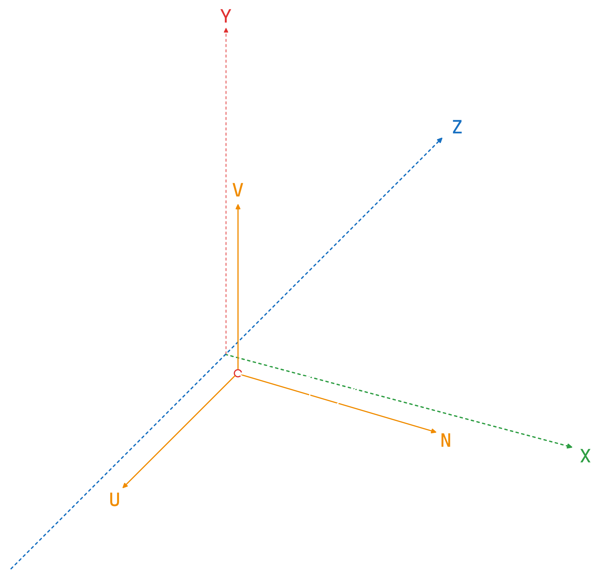
What do we want to achieve with the new 3D coordinate system is to align UVN with the XYZ of the world coordinate space. So U will be parallel to the X, V will be parallel to Y and N will be parallel to Z.
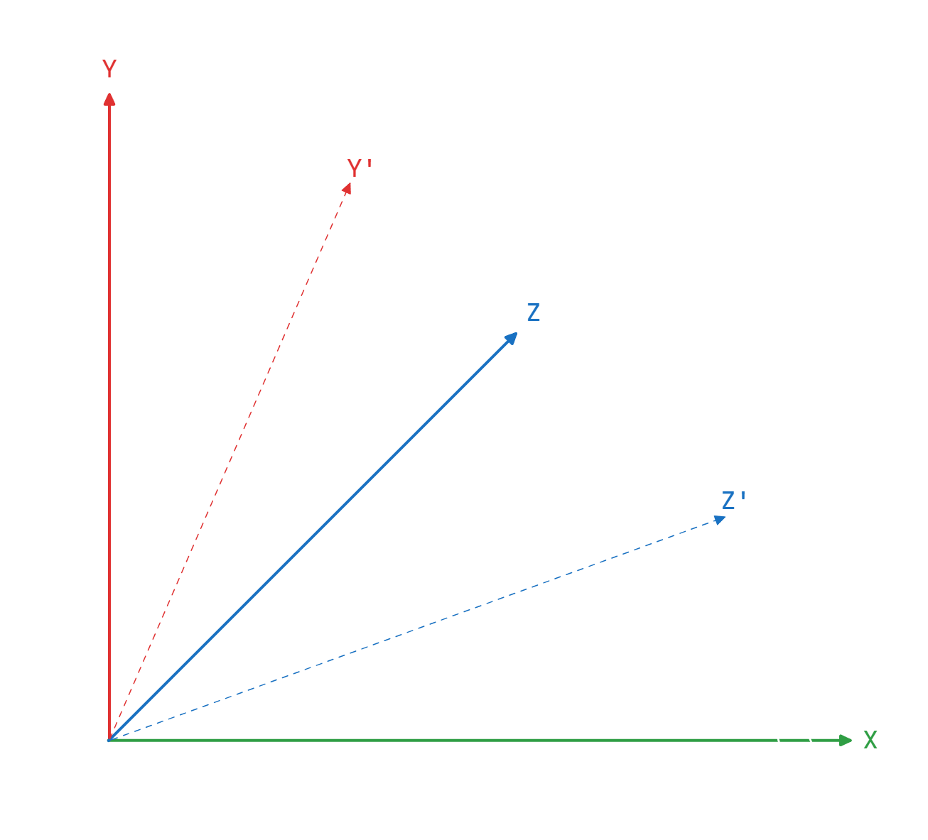
This means that if we have a vertex with position XYZ in the world coordinate system, we want to get its position X'Y'Z' in reference to the UVN coordinate system.
In other words, we need to apply a change of basis from the world coordinate system to the camera coordinate system to get the new object positions based in camera coordinate system.
Properties of UVN Model
The coordinate system conforming the UVN Model is linearly independent. That means that the axis are orthogonal to each other because they are 90 degrees between each two axis.
In addition, the axis are kept normalized because they are meant to be direction vectors, so length of each axis is always one.
Change of Basis
In order to understand how to perform a change of basis between coordinate systems, let's move to a 2D system sample as the core principle is the same.
A 2D point in the coordinate system for example v(2,3) can be represented as a multiplication of each component of the point by its corresponding coordinate axis like the following:
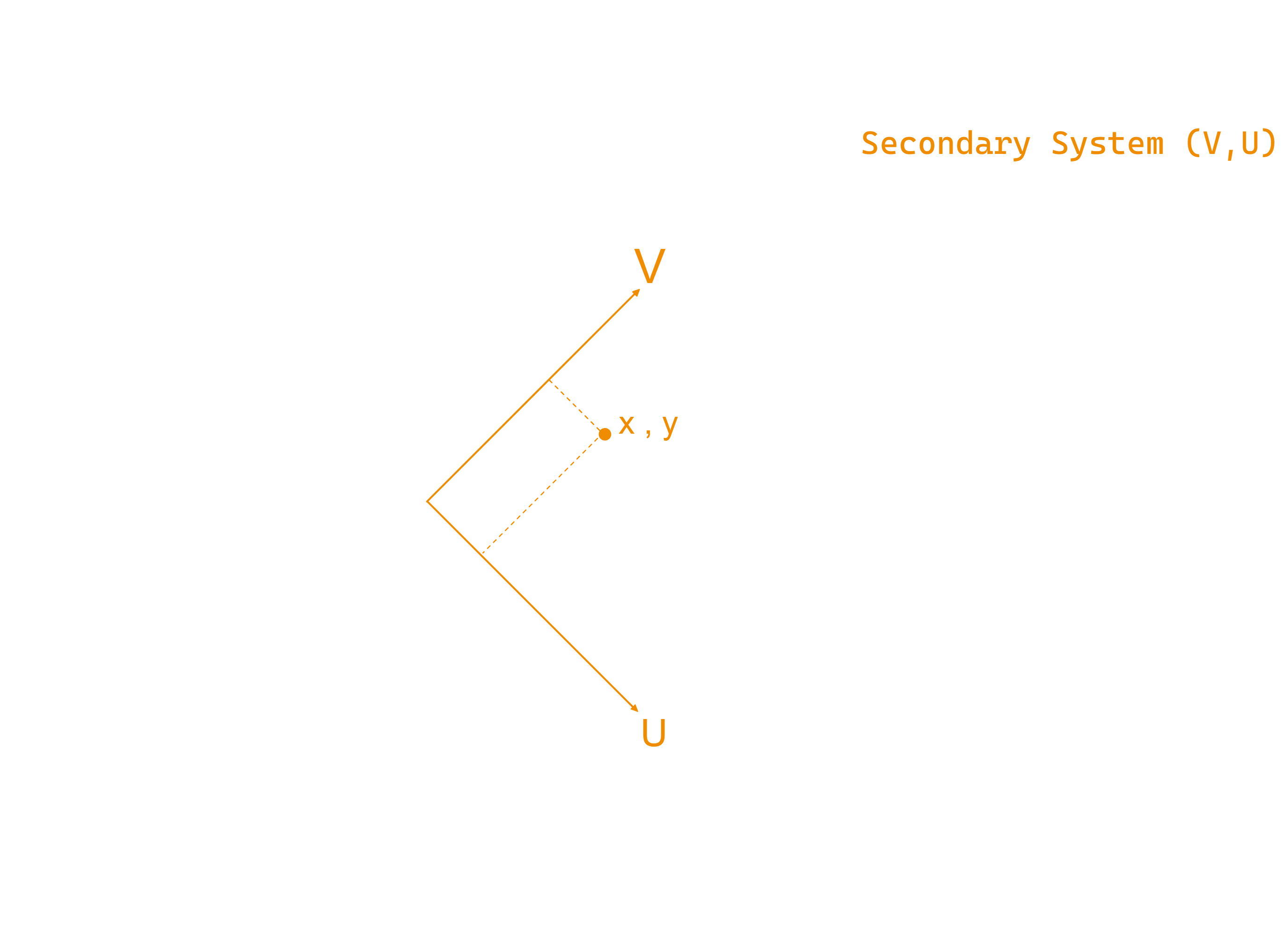
Knowing that, if we build a secondary coordinate system as a orthonormal axis given in the primary coordinate system, we can obtain any arbitrary 3D point that references to secondary coordinate system into the primary coordinate system.
Vector Transformation - Change of Basis
So if we have a position in coordinate system A, we can multiply each component by the corresponding axis using the coordinates of that axis in coordinate system B. We sum up all these products together and we get the position in coordinate system B.
Matrix Transformation - Change of Basis
Let's write the transformation in a matrix form. The axis of the secondary system in reference to the primary system are specified in columns forming the matrix.
When multiply the matrix by a position vector which is in reference to the secondary system we get the position in the primary system.
View Matrix
From now on, we have built the camera matrix based on UVN model in the world coordinate system.
As you might ask yourself, we know how to build new coordinate systems in the world coordinate system with the UVN Model and perform a change of basis in order to transform the 3D points of those new coordinate systems to the world coordinate system.
But, we need to do it in reverse, right? We need to go from the world system to the camera system since the objects are in world space and they should be in reference to the camera space in order to be in a valid range for the rasterizer.
The answer is applying the inverse of that matrix transformation, as we need to go from primary coordinate system (World) to secondary coordinate system (Camera).
Thus, we need to obtain the inverse matrix of the camera matrix.
As we know that multiplying the inverse of the matrix by the original matrix we obtain the identity matrix, we may use this equation to isolate and obtain the inverse matrix.
However, since the since the rows and columns of the transformation matrix are linearly independent and the length of vectors are one, we can just need to transpose the 3 by 3 submatrix where we put the UVN vectors.
On the other hand, we need to get the inverse of camera location to align the camera position to the origin of the primary coordinate system:
Lastly, we just need to perform a dot product of the inverse of camera location by each UVN vector to obtain the fourth column vector.
And that's the view matrix:
Code
The following code is an implementation of a view transformation where we define a new matrix method called View()
that recieves the camera matrix decomposed by its camera location 3D vector and its UVN model axis vectors (right, up, forward).
Those parameters are passed through the private method SetViewMatrix() to build the view matrix from the locally-created matrix.
Once we have the view matrix, we just need to perform the matrix-matrix multiplication using the new overwritted multiplication operator.
    void Matrix::View(const Vector3& aCamPos,
                       const Vector3& aRight, const Vector3& aUp, const Vector3& aForward)
    {
        // Creates an arbitrary matrix
        Matrix4 ViewMat {};

        // Set up as an identity matrix
        ViewMat.Indentiy();

        // Build the view matrix based on Camera Position and Camera orientation.
        ViewMat.SetViewMatrix(aCamPos, aCamRight, aCamUp, aCamForward);

        // Apply the perspective projection by matrix multiplication
        auto& MatRef = *this;
        MatRef = ViewMat * MatRef;
    }
In SetViewMatrix() private method, we set a transposed 3x3 matrix putting the UVN vectors inversely
and perform a dot product with the camera position vector to get the 4th column vector.
    void Matrix::SetViewMatrix(const Vector3& aCamPos,
                                const Vector3& aRight, const Vector3& aUp, const Vector3& aForward)
    {
        // Set up rotation submatrix transposing the UVN axis coords
        m_Mat[0]  = aRight.x;
        m_Mat[1]  = aUp.x;
        m_Mat[2]  = aForward.x;

        m_Mat[4]  = aRight.y;
        m_Mat[5]  = aUp.y;
        m_Mat[6]  = aForward.y;

        m_Mat[8]  = aRight.z;
        m_Mat[9]  = aUp.z;
        m_Mat[10] = aForward.z;

        // Build the translation submatrix by the dot product of position vector with UVN axis coords
        m_Mat[12] = -aRight.dot(aCamPos);
        m_Mat[13] = -aUp.dot(aCamPos);
        m_Mat[14] = -aForward.dot(aCamPos);
    }
In the Scene, we just need to use the View() method in order to build the view matrix.
In the example, we set up a UVN model rotated 45º counterclockwise from X axis and with a non-zero camera position.
    void Scene::OnUpdate()
    {
        // (1) Creating WizardMat and applying translation transform to visualize
        //     the 3D illusion through Z axis...
        // (2) Setting up ProjectionMat with the prespective params (FOV, aspect ratio, NearZ, FarZ)...

        // (3) Setting up CameraMat with the UVN model params (Position and UVN axis)
        Matrix4 CameraMat {};
        CameraMat.Identity();

        Vector3 CamPos      { 5.0f, 5.0f, 0.0f };
        Vector3 CamRight    { 0.5f, 0.0f, 0.5f };
        Vector3 CamUp       { 0.0f, 1.0f, 0.0f };
        Vector3 CamForward  {-0.5f, 0.0f, 0.5f };

        CameraMat.View(CamPos, CamRight, CamUp, CamForward);

        // (1) Send WizardMat to the GPU...
        // (2) Send ProjectionMat to the GPU...
        // (3) Send CameraMat to the GPU...
    }
If we run the sample code in our scene, we get something like this:
Coordinate Systems in 3D Graphics
To wrap up this amazing article about matrix transformation fundamentals, let's talk about the different coordinate systems that are involved in 3D graphics.
Coordinate System Pipeline
The following diagram summarizes all the transformations that are involved in 3D rendering:
-
Local Coordinate System: That's the coordinate system in which the models are created and when we talk about the position of vertices, we mean the position of the vertices in the local coordinate system. At this stage each model instance will be the same. -
World Coordinate System: We apply a world transformation including a combination of transformations such as scaling, rotation and translation on the vertices that moves them to their desired location in the world coordinate system. At this stage each model instance will be unique. -
View Coordinate System: Next, we apply a view or camera transformation. This moves them along with the camera to make it appear as if the camera is located at the origin and it is looking along the positive Z axis. -
Clip Coordinate System: Then, we apply perspective projection made up of the perspective projection matrix. At this point the vertices are in a clip coordinate system or clip space. -
Normalized Device coordinate System: Next, we perform perspective division. All the vertices that can be rendered are now in the range of -1 to 1 on all axes. We call this the normalized device coordinates, or NDC. -
Window Coordinate System: On the normalized device coordinates, we apply the viewport transform taking into account the aspect ratio of the screen which translates them to window coordinates. Now these are the actual pixels that can be rendered on the screen.

 Carlos Peña
